# Forecasting Crime Complaints in NYCC using GridDB and Python StatsModels
# Introduction
In this tutorial we will examine how to forecast the number of Crime Complaints in New York City by aggregating the data we ingested in the Nifi ETL tutorial and then using the statsmodels SARIMAX model to produce the forecast. The SARIMAX acronym stands for Seasonal Autoregressive Integrated Moving Average Exogenous and is an extension of ARIMA. The differences between the two are explained in this Machine Learning Mastery (opens new window) blog.
# Aggregating Data
We will perform two aggregations to maintain maximum flexibility in our forecasting, but first we will count the number of complaints in each precinct for every month in our examination period.
tqls=[]
dt =  datetime.datetime(2006, 1, 1, 0, 0, 0)
while dt < datetime.datetime(2016, 1, 1, 0, 0):
    start = int(dt.timestamp()*1000)
    end = int((dt + relativedelta(months=+1)).timestamp()*1000)
    query = "select count(*) where CMPLNT_FR > TO_TIMESTAMP_MS("+str(start)+")"
    query = query + " AND CMPLNT_FR < TO_TIMESTAMP_MS("+str(end)+")"
    tqls.append([dt, query])
    dt = dt + relativedelta(months=+1);
cols = []
for x in range(1, 125):
    col = gridstore.get_container("precinct_"+str(x))
    if col != None:
        cols.append([x, col])
for col in cols:
    for tql in tqls:
        q = col[1].query(tql[1])
        try:
            rs = q.fetch(False)
            if rs.has_next():
                data = rs.next()
                count = data.get(griddb.Type.LONG)
                print([str(col[0])+"_"+str(tql[0].timestamp()), tql[0], col[0], count ])
                aggcn.put([str(col[0])+"_"+str(tql[0].timestamp()), tql[0], col[0], count ])
        except:
            pass
As you can see, the aggregated data for each time bucket is written into a new container defined by the following schema:
conInfo = griddb.ContainerInfo("NYCC_AGGS",
                [["key", griddb.Type.STRING],
                ["timestamp", griddb.Type.TIMESTAMP],
                ["precinct", griddb.Type.INTEGER],
                ["count", griddb.Type.LONG]],
            griddb.ContainerType.COLLECTION, True)
aggcn = gridstore.put_container(conInfo)
As we are writing the aggregated data, this process only needs to be run once. The second aggregation will combine all of the different precincts' complaint counts into one total. This process only requires a few calculations and so there is no need to save the result.
tqls=[]
dt =  datetime.datetime(2006, 1, 1, 0, 0, 0)
while dt < datetime.datetime(2016, 1, 1, 0, 0):
    start = int((dt + relativedelta(days=-1)).timestamp()*1000)
    end = int((dt + relativedelta(days=+1)).timestamp()*1000)
    query = "select sum(count) where timestamp > TO_TIMESTAMP_MS("+str(start)+")"
    query = query + " AND timestamp < TO_TIMESTAMP_MS("+str(end)+")"
    tqls.append([dt, query])
    dt = dt + relativedelta(months=+1);
data = []
col = gridstore.get_container("NYCC_AGGS")
for tql in tqls:
        q = col.query(tql[1])
        rs = q.fetch(False)
        if rs.has_next():
            row = rs.next()
            count = row.get(griddb.Type.LONG)
            data.append([tql[0], count])
Now with all of the aggregates returned and put into a basic python list of lists, it needs to be transformed into a periodized Pandas dataframe that can be used with the SARIMAX model.
df = pd.DataFrame.from_records(data)
df = df.set_index(0)
ts = df[1]
ts = ts.to_period('M')
# Finding the Params
The first step in accurate time series forecasting is finding the order and seasonal order parameters that best fit the input data. The following loop iterates through all potential combinations and outputs Akaike information criterion (opens new window) (AIC) which estimates the quality of each model and its parameters.
    p = d = q = range(0, 2)
    pdq = list(itertools.product(p, d, q))
    seasonal_pdq = [(x[0], x[1], x[2], 12) for x in list(itertools.product(p, d, q))]
    sel_param=None
    sel_param_seasonal=None
    lowest_aic=None
    for param in pdq:
        for param_seasonal in seasonal_pdq:
            try:
                mod = sm.tsa.statespace.SARIMAX(ts,
                                            order=param,
                                            seasonal_order=param_seasonal,
                                            enforce_stationarity=False,
                                            enforce_invertibility=False)
                results = mod.fit()
                if lowest_aic == None or results.aic < lowest_aic:
                    sel_param = param
                    sel_param_seasonal = param_seasonal
                    lowest_aic = results.aic
            except:
                traceback.print_exc()
                continue
    print("Optimal param: ", sel_param, ", seasonal param:", sel_param_seasonal, " with AIC=",aic)
With this data set the optimal parameters were (1, 1, 1) and (1, 1, 1, 12) seasonal parameter.
# Forecasting
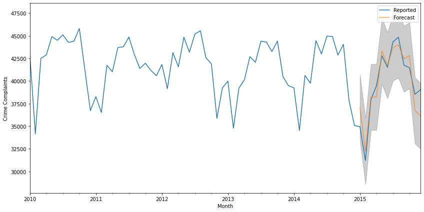
Now that we have chosen optimal parameters, we can run the SARIMAX model and plot the results.
mod = sm.tsa.statespace.SARIMAX(ts,
                            order=(1, 1, 1),
                            seasonal_order=(1, 1, 1, 12),
                            enforce_stationarity=False,
                            enforce_invertibility=False)
results = mod.fit()
print(results.summary().tables[1])
pred = results.get_prediction(start=pd.to_datetime('2015-01-01'), dynamic=False)
print(pred.predicted_mean)
pred_ci = pred.conf_int()
ax = ts['2010':].plot(label='Reported')
pred.predicted_mean.plot(ax=ax, label='Forecasted', alpha=.7, figsize=(14, 7))
ax.fill_between(pred_ci.index,
                pred_ci.iloc[:, 0],
                pred_ci.iloc[:, 1], color='k', alpha=.2)
ax.set_xlabel('Month')
ax.set_ylabel('Crime Complaints')
plt.legend()
plt.show()

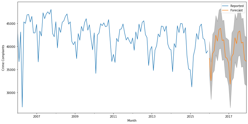
The above shows a forecast for data that we have fed into the model; the get_forecast function below returns the forecast for data points in the future which can also be plotted with its confidence interval (which grows as time progresses) as well.
pred_uc = results.get_forecast(steps=24)
pred_ci = pred_uc.conf_int()
ax = ts.plot(label='Reported', figsize=(14, 7))
pred_uc.predicted_mean.plot(ax=ax, label='Forecasted')
ax.fill_between(pred_ci.index,
                pred_ci.iloc[:, 0],
                pred_ci.iloc[:, 1], color='k', alpha=.25)
ax.set_xlabel('Month')
ax.set_ylabel('Crime Complaints')
plt.legend()
plt.show()

# Conclusion
With raw time series data stored in GridDB, it's easy to aggregate individual events into a set of counts that can be input into a Statsmodels SARIMAX model to predict forecast future events. The Jupyter Notebook (opens new window) used to calculate aggregations, find the ideal model parameters, and perform the forecast are available in the GridDB.net GitHub repository.
