Database function
Resource management
Besides the database residing in the memory, other resources constituting a GridDB cluster are perpetuated to a disk. The perpetuated resources are listed below.
Database file
A database file is a collective term for data files and checkpoint log files, where databases on the memory are periodically written to, and transaction log files that are saved every time data is updated.
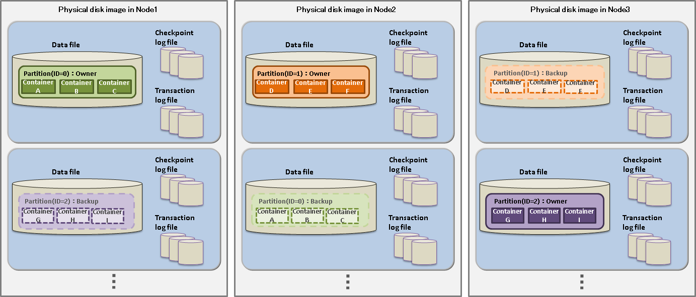
Data file
A checkpoint file is a file where partitions are persisted to a disk. Updated information is reflected in the memory by a cycle of the node definition file (/checkpoint/checkpointInterval). The file size expands relative to the data capacity. Once expanded, the size of a data file does not decrease even when data including container data and row data is deleted. In this case, GridDB reuses the free space instead. A data files can be split into smaller ones.
Checkpoint log file
A checkpoint log file is a file where block management information for partitions are persisted to a disk. Block management information is written in smaller batches at the interval (/checkpoint/checkpointInterval) specified in the node definition file. By default, a maximum of ten files are created for each partition. The number of split files can be adjusted by the number of batches (splits) /checkpoint/partialCheckpointInterval in the node definition file.
Transaction log file
Transaction data that are written to the database in memory is perpetuated to the transaction log file by writing the data sequentially in a log format. One file stores the logs of transactions executed from the start of the last checkpoint to the start of the next checkpoint. By default, a maximum of three files are created for each partition, consisting of the current log file and the previous two generations of log files.
Definition file
Definition file includes two types of parameter files: gs_cluster.json, hereinafter referred to as a cluster definition file, used when composing a cluster; gs_node.json, hereinafter referred to as a node definition file, used to set the operations and resources of the node in a cluster. It also includes a user definition file for GridDB administrator users.
Event log file
The event log of the GridDB server is saved in this file, including messages such as errors, warnings and so on.
Backup file
Backup data in the data file of GridDB is saved.
The placement of these resources is defined in GridDB home (path specified in environmental variable GS_HOME). In the initial installation state, the /var/lib/gridstore directory is GridDB home, and the initial data of each resource is placed under this directory.
The directories are placed initially as follows.
/var/lib/gridstore/        # GridDB home directory path
     admin/                # gs_admin home directory
     backup/               # Backup directory
     conf/                 # Definition files directory
          gs_cluster.json  # Cluster definition file
          gs_node.json     # Node definition file
          password         # User definition file
     data/                 # data files and checkpoint log directory
     txnlog/               # Transaction log directory
     expimp/               # Export/Import directory
     log/                  # Log directory
The location of GridDB home can be changed by setting the .bash_profile file of the OS user gsadm. If you change the location, please also move resources in the above directory accordingly.
The .bash_profile file contains two environment variables, GS_HOME and GS_LOG.
vi .bash_profile

# GridStore specific environment variables
GS_LOG=/var/lib/gridstore/log
export GS_LOG
GS_HOME=/var/lib/gridstore                    // GridDB home directory path
export GS_HOME
The database directory, backup directory and server event log directory can be changed by changing the settings of the node definition file as well.
See Parameters for the contents that can be set in the cluster definition file and node definition file.
Data access function
To access GridDB data, there is a need to develop an application using NoSQL I/F or NewSQL I/F. Data can be accessed simply by connecting to the cluster database of GridDB without having to take into account position information on where the container or table is located in the cluster database. The application system does not need to consider which node constituting the cluster the container is placed in.
In the GridDB API, when connecting to a cluster database initially, placement hint information of the container is retained (cached) on the client end together with the node information (partition).
Communication overheads are kept to a minimum as the node maintaining the container is connected and processed directly without having to access the cluster to search for nodes that have been placed every time the container used by the application is switched.
Although the container placement changes dynamically due to the rebalancing process in GridDB, the position of the container is transmitted as the client cache is updated regularly. For example, even when there is a node mishit during access from a client due to a failure or a discrepancy between the regular update timing and re-balancing timing, relocated information is automatically acquired to continue with the process.
TQL and SQL
TQL and SQL-92 compliant SQL are supported as database access languages.
What is TQL?
A simplified SQL prepared for GridDB SE. The support range is limited to functions such as search, aggregation, etc., using a container as a unit. TQL is employed by using the client API (Java, C language) of GridDB SE.
The TQL is adequate for the search in the case of a small container and a small number of hits. For that case, the response is faster than SQL. The number of hits can be suppressed by the LIMIT clause of TQL.
For the search of a large amount of data, SQL is recommended.
TQL is available for the containers and partitioned tables created by operations through the NewSQL interface. The followings are the limitations of TQL for the partitioned tables.
Filtering data by the WHERE clause is available. But aggregate functions, timeseries data selection or interpolation, min or max function and ORDER BY clause, etc. are not available.
It is not possible to apply the update lock.
What is SQL?
Standardization of the language specifications is carried out in ISO to support the interface for defining and performing data operations in conformance with SQL-92 in GridDB. SQL can be used in NewSQL I/F.
SQL is also available for the containers created by operations through the NoSQL interface.
Batch-processing function to multiple containers
An interface to quickly process event information that occurs occasionally is available in NoSQL I/F.
When a large volume of events is sent to the database server every time an event occurs, the load on the network increases and system throughput does not increase. Significant impact will appear especially when the communication line bandwidth is narrow. Multi-processing is available in NoSQL I/F to process multiple row registrations for multiple containers and multiple inquiries (TQL) to multiple containers with a single request. The overall throughput of the system rises as the database server is not accessed frequently.
An example is given below.
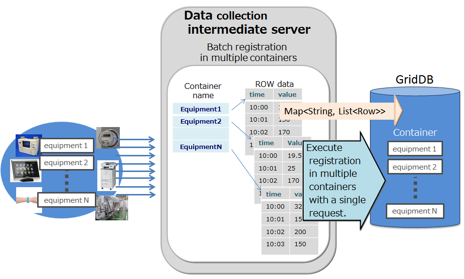
Multi-put
A container is prepared for each sensor name as a process to register event information from multiple sensors in the database. The sensor name and row array of the timeseries event of the sensor are created and a list (map) summarizing the data for multiple sensors is created. This list data is registered in the GridDB database each time the API is invoked.
Multi-put API optimizes the communication process by combining requests of data registration into multiple containers to a node in GridDB, which is formed by multiple clusters. In addition, multi-registrations are processed quickly without performing MVCC when executing a transaction.
In a multi-put processing, transactions are committed automatically. Data is confirmed on a single case basis.
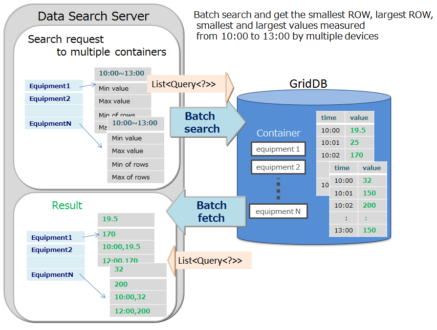
Multi-query (fetchAll)
- Instead of executing multiple queries to a container, these can be executed in a single query by aggregating event information of the sensor. For example, this is most suitable for acquiring aggregate results such as the daily maximum, minimum and average values of data acquired from a sensor, or data of a row set having the maximum or minimum value, or data of a row set meeting the specified condition.
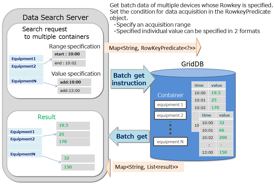
Multi-get
Instead of executing multiple queries to a sensor, these can be executed in a single query by consolidating event information of the sensor. For example, this is most suitable for acquiring aggregate results such as the daily maximum, minimum and average values of data acquired from a sensor, or data of a row set having the maximum or minimum value, or data of a row set meeting the specified condition.
In a RowKeyPredicate object, the acquisition condition is set in either one of the 2 formats below.
- Specify the acquisition range
- Specified individual value
Index function
A condition-based search can be processed quickly by creating an index for the columns of a container (table).
Two types of indexes are available: tree indexes (TREE) and spatial indexes (SPATIAL). The index that can be set differs depending on the container (table) type and column data type.
- TREE INDEX
- A tree index is used for an equality search and a range search (including greater than/equal to, and less than/equal to).
- This can be set for columns of the following data type in any type of container (table), except for columns corresponding to a rowkey in a timeseries container (timeseries table).
- STRING
- BOOL
- BYTE
- SHORT
- INTEGER
- LONG
- FLOAT
- DOUBLE
- TIMESTAMP
- Only a tree index allows an index with multiple columns, which is called a composite index. A composite index can be set up to 16 columns, where the same column cannot be specified more than once.
- SPATIAL INDEX
- Can be set for only GEOMETRY columns in a collection. This is specified when conducting a spatial search at a high speed.
Although there are no restrictions on the no. of indices that can be created in a container, creation of an index needs to be carefully designed. An index is updated when the rows of a configured container are inserted, updated or deleted. Therefore, when multiple indices are created in a column of a row that is updated frequently, this will affect the performance in insertion, update or deletion operations.
An index is created in a column as shown below.
- A column that is frequently searched and sorted
- A column that is frequently used in the condition of the WHERE section of TQL
- High cardinality column (containing few duplicated values)
[Note]
- Only a tree index can be set to the column of a table (time series table).
Function specific to time series data
To manage data frequently produced from sensors, data is placed in accordance with the data placement algorithm (TDPA: Time Series Data Placement Algorithm), which allows the best use of the memory. In a timeseries container (timeseries table), memory is allocated while classifying internal data by its periodicity. When hint information is given in an affinity function, the placement efficiency rises further. Moreover, a timeseries container moves data out to a disk if necessary and releases expired data at almost zero cost.
A timeseries container (timeseries table) has a TIMESTAMP ROWKEY (PRIMARY KEY).
Operation function of TQL
Aggregate operations
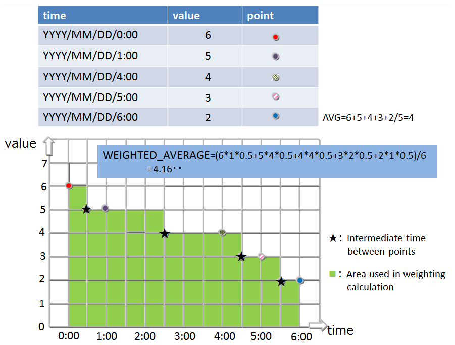
In a timeseries container (timeseries table), the calculation is performed with the data weighted at the time interval of the sampled data. In other words, if the time interval is long, the calculation is carried out assuming the value is continued for an extended time.
The functions of the aggregate operation are as follows:
TIME_AVG
- TIME_AVG Returns the average weighted by a time-type key of values in the specified column.
- The weighted average is calculated by dividing the sum of products of sample values and their respective weighted values by the sum of weighted values. The method for calculating a weighted value is as shown above.
- The details of the calculation method are shown in the figure:
Selection/interpolation operation
Time data may deviate slightly from the expected time due to the timing of the collection and the contents of the data to be collected. Therefore when conducting a search using time data as a key, a function that allows data around the specified time to be acquired is also required.
The functions for searching the timeseries container (timeseries table) and acquiring the specified row are as follows:
TIME_NEXT(*, timestamp)
Selects a time-series row whose timestamp is identical with or just after the specified timestamp.
TIME_NEXT_ONLY(*, timestamp)
Select a time-series row whose timestamp is just after the specified timestamp.
TIME_PREV(*, timestamp)
Selects a time-series row whose timestamp is identical with or just before the specified timestamp.
TIME_PREV_ONLY(*, timestamp)
Selects a time-series row whose timestamp is just before the specified timestamp.
In addition, the functions for interpolating the values of the columns are as follows:
TIME_INTERPOLATED(column, timestamp)
Returns a specified column value of the time-series row whose timestamp is identical with the specified timestamp, or a value obtained by linearly interpolating specified column values of adjacent rows whose timestamps are just before and after the specified timestamp, respectively.
TIME_SAMPLING(*|column, timestamp_start, timestamp_end, interval, DAY|HOUR|MINUTE|SECOND|MILLISECOND)
Takes a sampling of Rows in a specific range from a given start time to a given end time.
Each sampling time point is defined by adding a sampling interval multiplied by a non-negative integer to the start time, excluding the time points later than the end time.
If there is a Row whose timestamp is identical with each sampling time point, the values of the Row are used. Otherwise, interpolated values are used.
Expiry release function
An expiry release is a function to delete expired row data from GridDB physically. The data becomes unavailable by removing from a target for a search or a delete before deleting. Deleting old unused data results to keep database size results in prevention of performance degradation caused by bloat of database size.
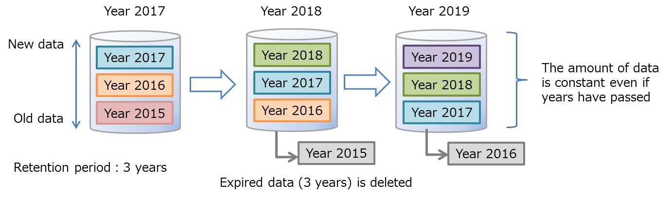
The retention period is set in container units. The row which is outside the retention period is called "expired data." The APIs become unable to operate expired data because it becomes unavailable. Therefore, applications can not access the row. Expired data will be the target for being deleted physically from GridDB after a certain period. Cold data is automatically removed from database intact.
Expiry release settings
Expiry release can be used in a partitioned container (table).
- It can be set for the following tables partitioned by interval and interval-hash.
- Timeseries table
- Collection table with a TIMESTAMP-type partitioning key
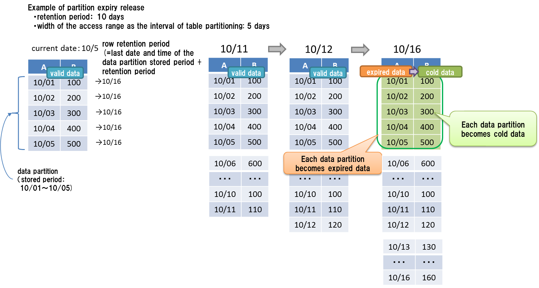
- Setting items consist of a retention period and a retention period unit.
- The retention period unit can be set in day/hour/minute/sec/millisecond units. The year unit and month unit cannot be specified.
- The expiration date of rows is calculated by adding the last date and time of the row stored period in the partition to the retention period. The rows stored in the same data partition have the same expiration date.
- The unit becoming cold data is a data partition. Physical data delete is executed on a data partition basis.
[Note]
Expiry release should be set when creating a table. They cannot be changed after creation.
The current time used for judging expiration depends on the environment of each node of GridDB. Therefore, because of the network latency or time difference of the execution environments, you may not be able to access the rows in a GridDB node whose environment time is ahead of that of the client you use; on the contrary, you may be able to access the rows if the client you use is ahead of the time of GridDB. You had better set the period a larger value than you need to avoid unintentional loss of rows.
The expired rows are separated from the object of search and updating, being treated as not to exist in the GridDB. Operations to the expired row do not cause errors.
- For example, for settings with an expiration of 30 days, even when a row with a timestamp of 31 days before the present date is registered, registration processing does not lead to an error, while the row is not saved in the table.
When you set up expiry release, be sure to synchronize the environment time of all the nodes of a cluster. If the time is different among the nodes, the expired data may not be released at the same time among the nodes.
The period that expired data becomes cold data depends on the setting of the retention period in the expiry release.
Retention period Max period that expired data becomes cold data -3 days about 1.2 hours 3 days-12 days about 5 hours 12 days-48 days about 19 hours 48 days-192 days about 3 days 192 days-768 days about 13 days 768 days- about 38 days
Automatic deletion of cold data or save as an archive
The management information for database files are periodically scanned every one second, and a row that has become cold data at the time of scanning is physically deleted. The amount of scanning the management information for database files is 2000 blocks per execution. It can be set /dataStore/batchScanNum in the node definition file (gs_node.json). There is a possibility that the size of DB keeps increasing because the speed of automatic deletion is behind one of registration in the system which data are registered frequently. Increase the amount of scanning to avoid it.
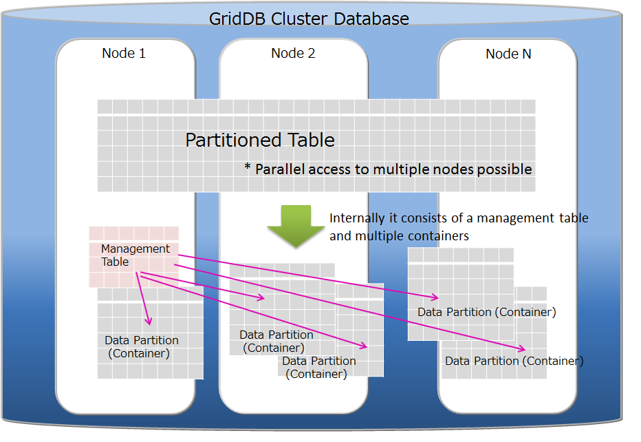
Table partitioning function
In order to improve the operation speed of applications connected to multiple nodes of the GridDB cluster, it is important to arrange the data to be processed in memory as much as possible. For a huge container (table) with a large number of registered data, the CPU and memory resources in multiple nodes can be effectively used by splitting data from the table and distributing the data across nodes. Distributed rows are stored in the internal containers called "data partition". The allocation of each row to the data partition is determined by a "partitioning key" column specified at the time of the table creation.
GridDB supports hash partitioning, interval partitioning and interval-hash partitioning as table partitioning methods.
Creating and Deleting tables can be performed only through the NewSQL interface. Data registration, update and search can be performed through the NewSQL/NoSQL interface. (There are some restrictions. See TQL Reference for the details.)
Data registration
When data is registered into a table, the data is stored in the appropriate data partition according to the partitioning key value and the partitioning method. It is not possible to specify a data partition to be stored.
Index
When creating an index on a table, a local index for each data partition is created. It is not possible to create a global index for the whole table.
Data operation
An error occurs for updating the partitioning key value of the primary key column. If updating is needed, delete and reregister the data.
Updating the partitioning key value of the not primary key column can be executed through NoSQL I/F.
Expiry release function
Expiry release can be set for the following tables partitioned by interval and interval-hash.
- Timeseries table
- Collection table with a TIMESTAMP-type partitioning key
Notes
Starting with V4.3, specifying a column other than the primary key as a partitioning key when the primary key does exist generates an error by default. To avoid this error, set false to /sql/partitioningRowkeyConstraint in the cluster definition file (gs_cluster.json).
When specifying the column as a partitioning key other than the primary key, the primary key constraint is ensured in each data partition, but it is not ensured in the whole table. So, the same value may be registered in multiple rows of a table.
Benefits of table partitioning
Dividing a large amount of data through a table partitioning is effective for efficient use of memory and for performance improvement in data search which can select the target data.
efficient use of memory
In data registration and search, data partitions required for the processing are loaded into memory. Other data partitions, not target to the processing, are not loaded. So when the data to be processed is locally concentrated on some data partitions, the amount of loading data is reduced. The frequency of swap-in and swap-out is decreased and the performance is upgraded.
selecting target data in data search
In data search, only data partitions matching the search condition are selected as the target data. Unnecessary data partitions are not accessed. This function is called "pruning". Because the amount of accessed data reduces, the search performance is upgraded. Search conditions which can enable the pruning are different depending on the type of the partitioning.
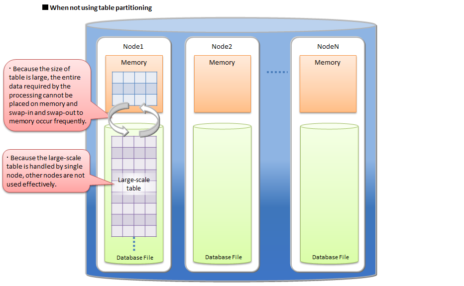
The followings describe the behaviors on the above items for both cases in not using the table partitioning and in using the table partition.
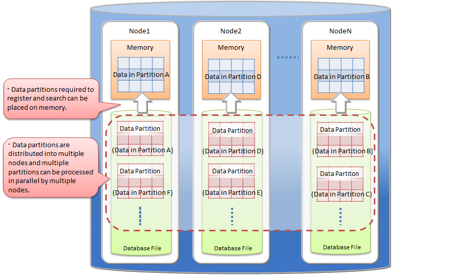
When a large amount of data is stored in single table which is not partitioned, all the required data might not be able to be placed on main memory and the performance might be degraded by frequent swap-in and swap-out between database files and memory. Particularly the degradation is significant when the amount of data is much larger than the memory size of a GridDB node. And data accesses to that table concentrate on single node and the parallelism of database processing decreases.
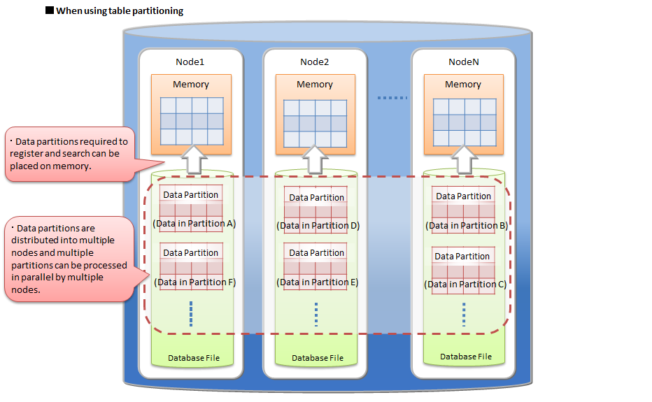
By using a table partitioning, the large amount of data is divided into data partitions and those partitions are distributed on multiple nodes.
In data registration and search, only necessary data partitions for the processing can be loaded into memory. Data partitions not target to the processing are not loaded. Therefore, in many cases, data size required by the processing is smaller than for a not partitioned large table and the frequency of swap-in and swap-out decreases. By dividing data into data partitions equally, CPU and memory resource on each node can be used more effectively.
In addition data partitions are distributed on nodes, so parallel data access becomes possible.
Hash partitioning
The rows are evenly distributed in the data partitions based on the hash value.
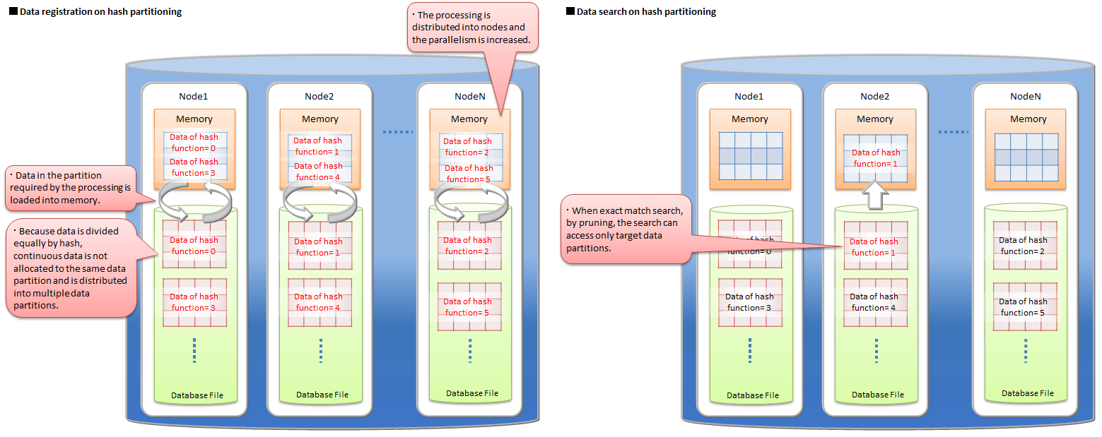
Also, when using an application system that performs data registration frequently, the access will concentrate at the end of the table and may lead to a bottleneck. A hash function that returns an integer from 1 to N is defined by specifying the partition key column and division number N, and division is performed based on the returned value.
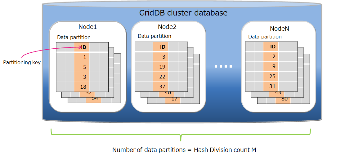
Data partitioning
By specifying the partitioning key and the division count M, a hash function that returns 1-M is defined, and data partitioning is performed by the hash value. The maximum hash value is 1024.
Partitioning key
There is no limitation for the column type of a partitioning key.
Creation of data partitions
Specified number of data partitions are created automatically at the time of the table creation. It is not possible to change the number of data partitions. The table re-creation is needed for changing the number.
Deletion of a table
It is not possible to delete only a data partition.
By deleting a hash partitioned table, all data partitions that belong to it are also deleted
Pruning
In key match search on hash partitioning, by pruning, the search accesses only data partitions which match the condition. So the hash partitioning is effective for performance improvement and memory usage reduction in that case.
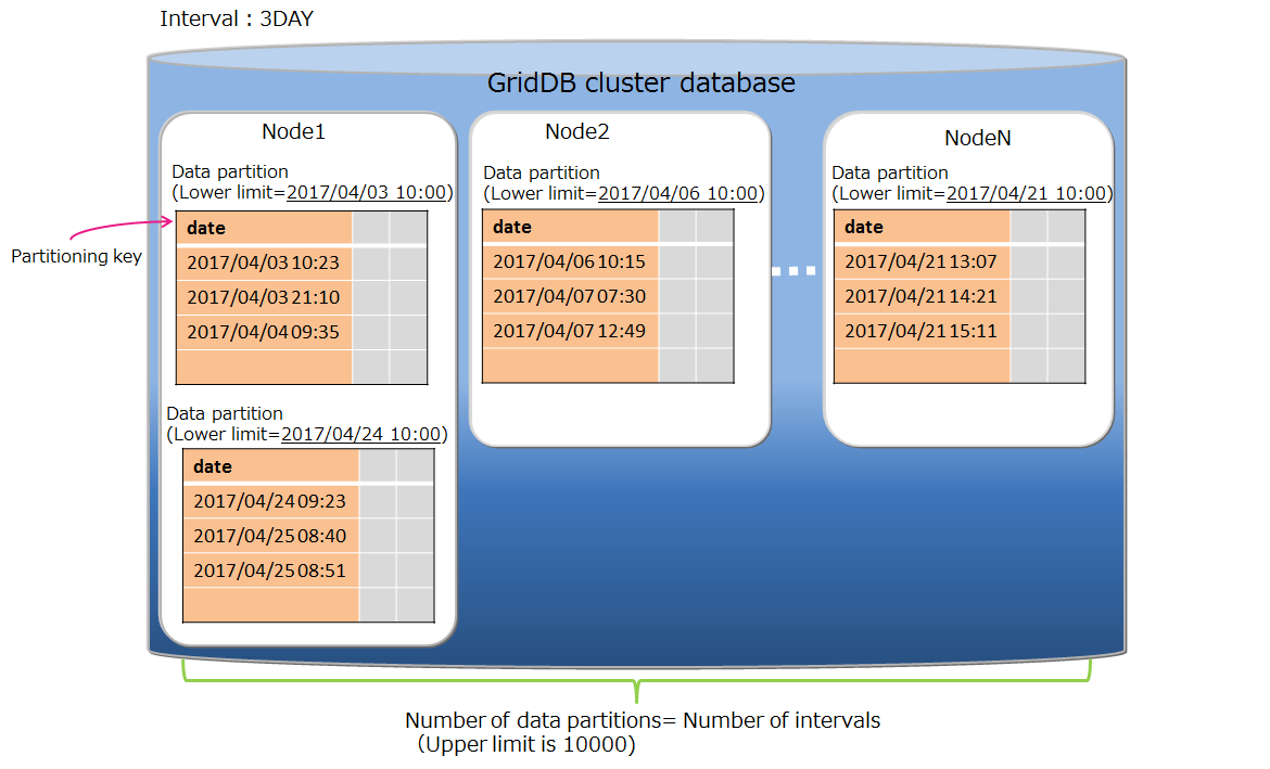
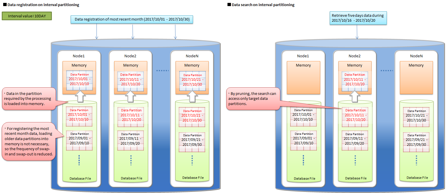
Interval partitioning
In the interval partitioning, the rows in a table are divided by the specified interval value and is stored in data partitions. The range of each data partition (from the lower limit value to the upper limit value) is automatically determined by the interval value.
The data in the same range are stored in the same data partition, so for the continuous data or for the range search, the operations can be performed on fewer memory.
Data partitioning
Data partitioning is performed by the interval value. The possible interval values are different depending on the partitioning key type.
- BYTE type : from 1 to 27-1
- SHORT type : from 1 to 215-1
- INTEGER type : from 1 to 231-1
- LONG type : from 1000 to 263-1
- TIMESTAMP: more than 1
When the partitioning key type is TIMESTAMP, it is necessary to specify the interval unit as 'DAY'.
Partitioning key
Data types that can be specified as a partitioning key are BYTE, SHORT, INTEGER, LONG and TIMESTAMP. The partitioning key is a column that needs to have "NOT NULL" constraint.
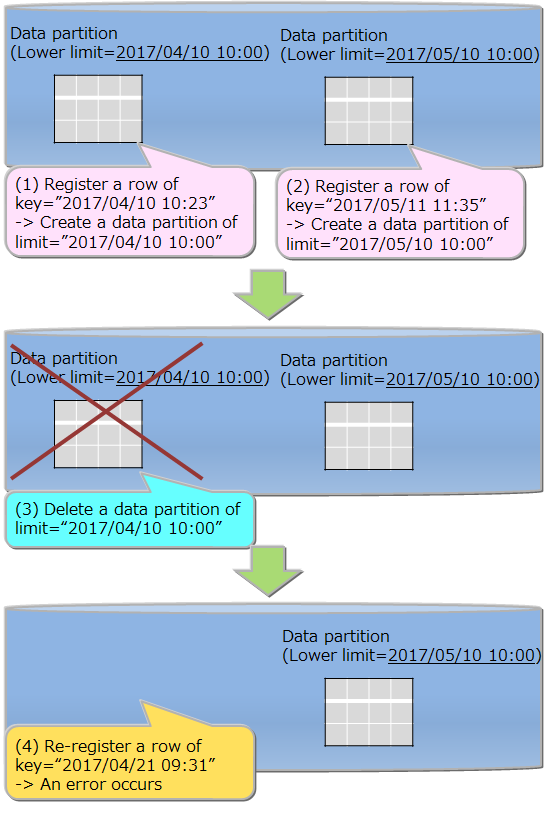
Creation of data partitions
Data partitions are not created at the time of creating the table. When there is no data partition for the registered row, a new data partition is automatically created.
The upper limit of the number of the data partitions is 10000. When the number of the data partitions reaches the limit, the data registration that needs to create a new data partition causes an error. For that case, delete unnecessary data partitions and reregister the data.
It is desired to specify the interval value by considering the range of the whole data and the upper limit, 10000, for the number of data partitions. If the interval value is too small to the range of the whole data and too many data partitions are created, the maintenance of deleting unnecessary data partitions is required frequently.
Deletion of a table
Each data partition can be deleted. The data partition that has been deleted cannot be recreated. All registration operations to the deleted data partition cause an error. Before deleting the data partition, check its data range by a metatable.
By deleting an interval partitioned table, all data partitions that belong to it are also deleted.
All data partitions are processed for the data search on the whole table, so the search can be performed efficiently by deleting unnecessary data partitions beforehand.
Maintenance of data partitions
In the case of reaching the upper limit, 10000, for the number of data partitions or existing unnecessary data partitions, the maintenance by deleting data partitions is needed.
Pruning
By specifying a partitioning key as a search condition in the WHERE clause, the data partitions corresponding the specified key are only referred for the search, so that the processing speed and the memory usage are improved.
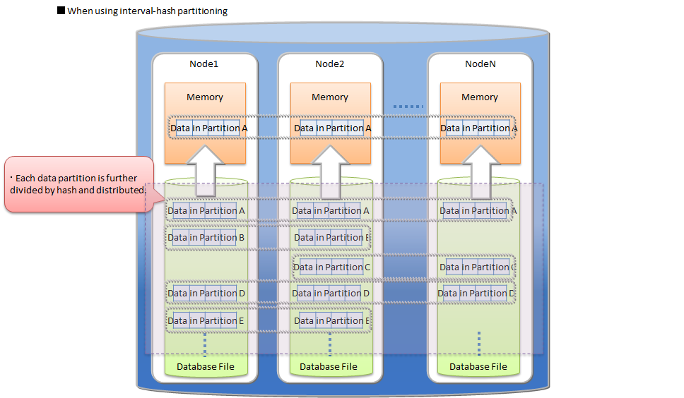
Interval-hash partitioning
The interval-hash partitioning is a combination of the interval partitioning and the hash partitioning. First the rows are divided by the interval partitioning, and further each division is divided by hash partitioning. The number of data partitions is obtained by multiplying the interval division count and the hash division count together.
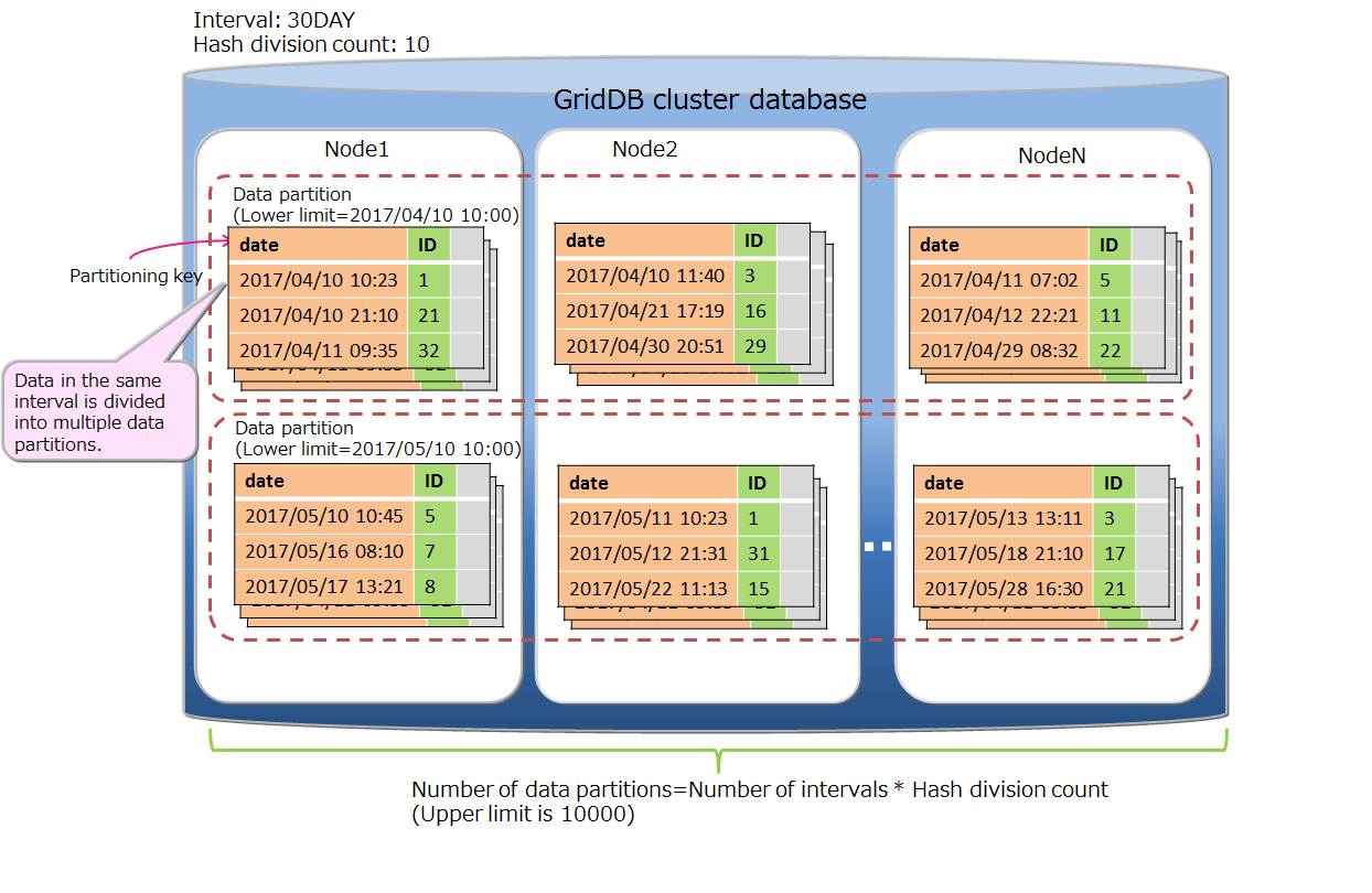
The rows are distributed to multiple nodes appropriately through the hash partitioning on the result of the interval partitioning. On the other hand, the number of data partitions increases, so that the overhead of searching on the whole table also increases. Please judge to use the partitioning by considering its data distribution and search overhead.
The basic functions of the interval-hash partitioning are the same as the functions of interval partitioning and the hash partitioning. The items specific for the interval-hash partitioning are as follows.
Data partitioning
The possible interval values of LONG are different from the interval partitioning.
- BYTE type : from 1 to 27-1
- SHORT type : from 1 to 215-1
- INTEGER type : from 1 to 231-1
- LONG type : from 1000 * hash division count to 263-1
- TIMESTAMP: more than 1
Number of data partitions
Including partitions divided by hash, the upper limit of number of data partitions is 10000. The behavior and requiring maintenance when the limit has been reached are same as interval partitioning.
Deletion of a table
A group of data partitions which have the same range can be deleted. It is not possible to delete only a data partition divided by the hash partitioning.
Selection criteria of table partitioning type
Hash, interval and interval-hash are supported as a type of table partitioning by GridDB.
A column which is used in conditions of search or data access must be specified as a partitioning key for dividing the table. If a width of range that divides data equally can be determined for values of the partitioning key, interval or interval-hash is suitable. Otherwise hash should be selected.
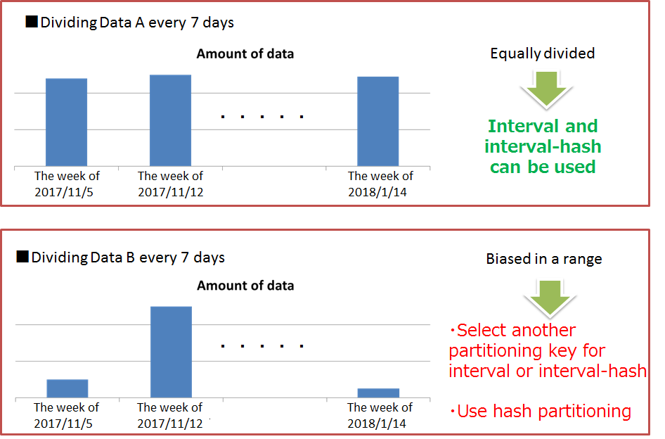
Interval partitioning, interval-hash partitioning
If an interval, a width of range to divide data equally, can be determined beforehand, interval partitioning is suitable. In the query processing on interval partitioning, by partitioning pruning, the result is acquired from only the data partitions matching the search condition, so the performance is improved. Besides the query processing, when registering successive data in a specific range, performance is improved.
Therefore, when using interval partitioning, by selecting an appropriate interval value based on frequently registered or searched data range in application programs, required memory size is reduced. For example, in the case of a system in which time-series data such as sensor data is frequently searched for the latest data, if the search target range is the division width value of interval partitioning, the search is performed in the memory of the data partition size to be processed and the performance dose not deteriorates.
Further by using interval-hash partitioning, data in each interval is distributed to multiple nodes equally, so accesses to the same data partition can also be performed in parallel.
Hash partitioning
When the characteristics of data to be stored is not clear or finding the interval value, which can divide the data equally, is difficult, hash partitioning should be selected. By specifying a column holding unique values as a partitioning key, uniform partitioning for a large amount of data is performed automatically.
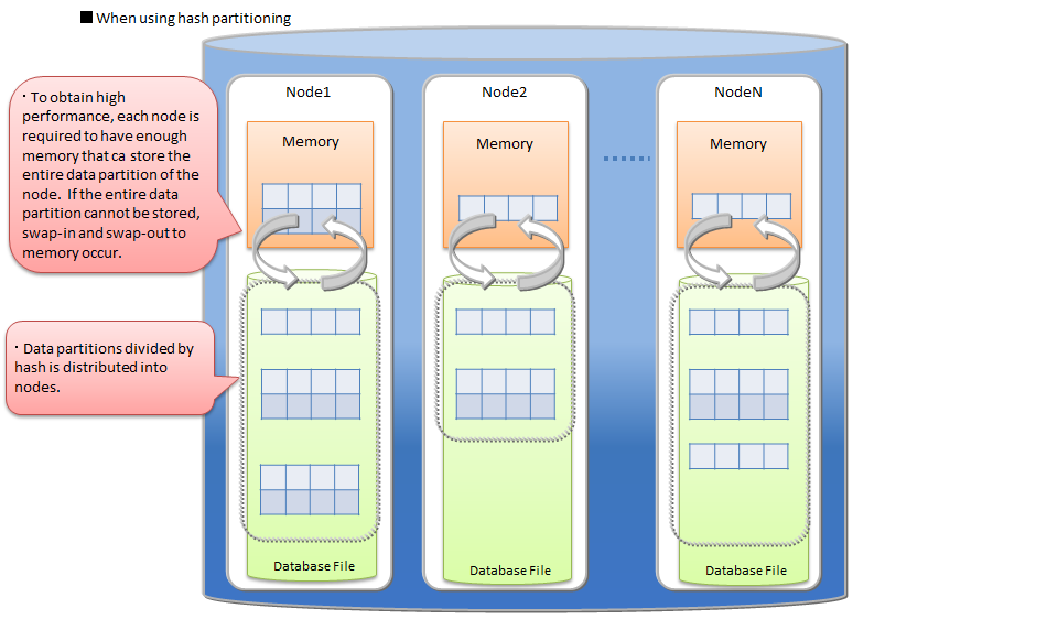
When using hash partitioning, the parallel access to the entire table and the partitioning pruning which is enabled only for exact match search can be performed, so the system performance can be improved. But, to obtain high performance, each node is required to have enough memory that can store the entire data partition of the node.
Transaction function
GridDB supports transaction processing on a container basis and ACID characteristics which are generally known as transaction characteristics. The supporting functions in a transaction process are explained in detail below.
Starting and ending a transaction
When a row search or update etc. is carried out on a container, a new transaction is started and this transaction ends when the update results of the data are committed or aborted.
[Note]
- A commit is a process to confirm transaction information under processing to perpetuate the data.
- In GridDB, updated data of a transaction is stored as a transaction log by a commit process, and the lock that had been maintained will be released.
- An abort is a process to rollback (delete) all transaction data under processing.
- In GridDB, all data under processing are discarded and retained locks will also be released.
The initial action of a transaction is set in autocommit.
In autocommit, a new transaction is started every time a container is updated (data addition, deletion or revision) by the application, and this is automatically committed at the end of the operation. A transaction can be committed or aborted at the requested timing by the application by turning off autocommit.
A transaction recycle may terminate in an error due to a timeout in addition to being completed through a commit or abort. If a transaction terminates in an error due to a timeout, the transaction is aborted. The transaction timeout is the elapsed time from the start of the transaction. Although the initial value of the transaction timeout time is set in the definition file (gs_node.json), it can also be specified as a parameter when connecting to GridDB on an application basis.
Transaction consistency level
There are 2 types of transaction consistency levels, immediate consistency and eventual consistency. This can also be specified as a parameter when connecting to GridDB for each application. The default setting is immediate consistency.
immediate consistency
- Container update results from other clients are reflected immediately at the end of the transaction concerned. As a result, the latest details can be referenced all the time.
eventual consistency
- Container update results from other clients may not be reflected immediately at the end of the transaction concerned. As a result, there is a possibility that old details may be referred to.
Immediate consistency is valid in update operations and read operations. Eventual consistency is valid in read operations only. For applications which do not require the latest results to be read all the time, the reading performance improves when eventual consistency is specified.
Transaction isolation level
Conformity of the database contents need to be maintained all the time. When executing multiple transaction simultaneously, the following events will generally surface as issues.
Dirty read
An event which involves uncommitted data written by a dirty read transaction being read by another transaction.
Non-repeatable read
An event which involves data read previously by a non-repeatable read transaction becoming unreadable. Even if you try to read the data read previously by a transaction again, the previous data can no longer be read as the data has already been updated and committed by another transaction (the new data after the update will be read instead).
Phantom read
An event in which the inquiry results obtained previously by a phantom read transaction can no longer be acquired. Even if you try to execute an inquiry executed previously in a transaction again in the same condition, the previous results can no longer be acquired as the data satisfying the inquiry condition has already been changed, added and committed by another transaction (new data after the update will be acquired instead).
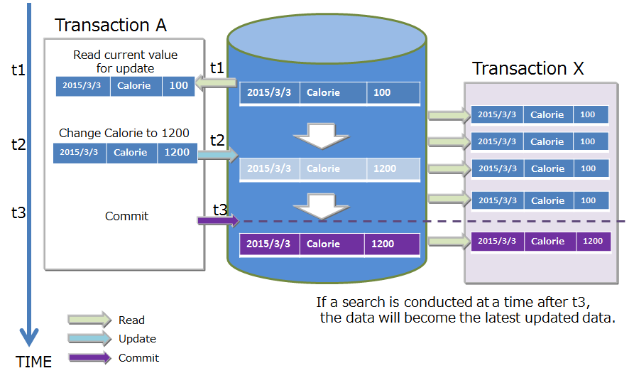
In GridDB, "READ_COMMITTED" is supported as a transaction isolation level. In READ_COMMITTED, the latest data confirmed data will always be read.
When executing a transaction, this needs to be taken into consideration so that the results are not affected by other transactions. The isolation level is an indicator from 1 to 4 that shows how isolated the executed transaction is from other transactions (the extent that consistency can be maintained).
The 4 isolation levels and the corresponding possibility of an event raised as an issue occurring during simultaneous execution are as follows.
| Isolation level | Dirty read | Non-repeatable read | Phantom read |
|---|---|---|---|
| READ_UNCOMMITTED | Possibility of occurrence | Possibility of occurrence | Possibility of occurrence |
| READ_COMMITTED | Safe | Possibility of occurrence | Possibility of occurrence |
| REPEATABLE_READ | Safe | Safe | Possibility of occurrence |
| SERIALIZABLE | Safe | Safe | Safe |
In READ_COMMITED, if data read previously is read again, data that is different from the previous data may be acquired, and if an inquiry is executed again, different results may be acquired even if you execute the inquiry with the same search condition. This is because the data has already been updated and committed by another transaction after the previous read.
In GridDB, data that is being updated by MVCC is isolated.
MVCC
In order to realize READ_COMMITTED, GridDB has adopted "MVCC (Multi-Version Concurrency Control)".
MVCC is a processing method that refers to the data prior to being updated instead of the latest data that is being updated by another transaction when a transaction sends an inquiry to the database. System throughput improves as the transaction can be executed concurrently by referring to the data prior to the update.
When the transaction process under execution is committed, other transactions can also refer to the latest data.
Lock
There is a data lock mechanism to maintain the consistency when there are competing container update requests from multiple transactions.
The lock granularity differs depending on the type of container. In addition, the lock range changes depending on the type of operation in the database.
Lock granularity
The lock granularity for each container type is as follows.
- Collection: Lock by ROW unit.
- Timeseries container: Locked by ROW collection
- In a ROW collection, multiple rows are placed in a timeseries container by dividing a block into several data processing units. This data processing unit is known as a row set. It is a data management unit to process a large volume of timeseries containers at a high speed even though the data granularity is coarser than the lock granularity in a collection.
These lock granularity were determined based on the use-case analysis of each container type.
- Collection data may include cases in which an existing ROW data is updated as it manages data just like a RDB table.
- A timeseries container is a data structure to hold data that is being generated with each passing moment and rarely includes cases in which the data is updated at a specific time.
Lock range by database operations
Container operations are not limited to just data registration and deletion but also include schema changes accompanying a change in data structure, index creation to improve speed of access, and other operations. The lock range depends on either operations on the entire container or operations on specific rows in a container.
Lock the entire container
- Index operations (createIndex/dropIndex)
- Deleting container
- Schema change
Lock in accordance with the lock granularity
- put/update/remove
- get(forUpdate)
In a data operation on a row, a lock following the lock granularity is ensured.
If there is competition in securing the lock, the subsequent transaction will be put in standby for securing the lock until the earlier transaction has been completed by a commit or rollback process and the lock is released.
A standby for securing a lock can also be cancelled by a timeout besides completing the execution of the transaction.
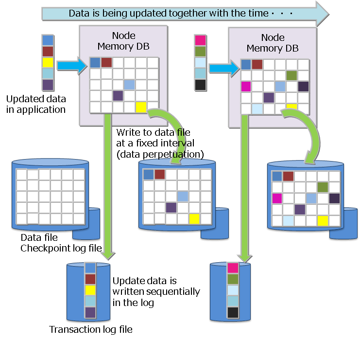
Data perpetuation
Data registered or updated in a container or table is perpetuated in the disk or SSD, and protected from data loss when a node failure occurs. In data persistence, there are two processes: one is a checkpoint process for periodically saving the updated data on the memory in data files and checkpoint log files for each block, and the other is a transaction log process for sequentially writing the updated data to transaction log files in sync with data updates.
To write to a transaction log, either one of the following settings can be made in the node definition file.
- 0: SYNC
- An integer value of 1 or higher: DELAYED_SYNC
In the "SYNC" mode, log writing is carried out synchronously every time an update transaction is committed or aborted. In the "DELAYED_SYNC" mode, log writing during an update is carried out at a specified delay of several seconds regardless of the update timing. Default value is "1 (DELAYED_SYNC 1 sec)".
When "SYNC" is specified, although the possibility of losing the latest update details when a node failure occurs is lower, the performance is affected in systems that are updated frequently.
On the other hand, if "DELAYED_SYNC" is specified, although the update performance improves, any update details that have not been written in the disk when a node failure occurs will be lost.
If there are 2 or more replicas in a raster configuration, the possibility of losing the latest update details when a node failure occurs is lower even if the mode is set to "DELAYED_SYNC" as the other nodes contain replicas. Consider setting the mode to "DELAYED_SYNC" as well if the update frequency is high and performance is required.
In a checkpoint, the update block is updated in the database file. A checkpoint process operates at the cycle set on a node basis. A checkpoint cycle is set by the parameters in the node definition file. Initial value is 60 sec (1 minute).
By raising the checkpoint execution cycle figure, data perpetuation can be set to be carried out in a time band when there is relatively more time to do so e.g. by perpetuating data to a disk at night and so on. On the other hand, when the cycle is lengthened, the disadvantage is that the number of transaction log files that have to be rolled forward when a node is restarted outside the system process increases, thereby increasing the recovery time.
Timeout process
NoSQL I/F and a NewSQL I/F have different setting items for timeout processing.
NoSQL I/F timeout process
In the NoSQL I/F, 2 types of timeout could be notified to the application developer, Transaction timeout and Failover timeout. The former is related to the processing time limit of a transaction, and the latter is related to the retry time of a recovery process when a failure occurs.
TransactionTimeout
The timer is started when access to the container subject to the process begins, and a timeout occurs when the specified time is exceeded.
Transaction timeout is configured to delete lock, and memory from a long-duration update lock (application searches for data in the update mode, and does not delete when the lock is maintained) or a transaction that maintains a large amount of results (application does not delete the data when the lock is maintained). Application process is aborted when transaction timeout is triggered.
A transaction timeout time can be specified in the application with a parameter during cluster connection. The upper limit of this can be specified in the node definition file. The default value of upper limit is 300 seconds. To monitor transactions that take a long time to process, enable the timeout setting and set a maximum time in accordance with the system requirements.
FailoverTimeout
Timeout time during an error retry when a client connected to a node constituting a cluster which failed connects to a replacement node. If a new connection point is discovered in the retry process, the client application will not be notified of the error. Failover timeout is also used in timeout during initial connection.
A failover timeout time can be specified in the application by a parameter during cluster connection. Set the timeout time to meet the system requirements.
Both the transaction timeout and failover timeout can be set when connecting to a cluster using a GridDB object in the Java API or C API.
NewSQL I/F timeout process
There are 3 types of timeout as follows:
Login (connection) timeout
Timeout for initial connection to the cluster. The default value is 300 seconds (5 minutes) and can be changed using DriverManager of API .
Network timeout
Timeout in response between client and cluster. The timeout time is 300 seconds (5 minutes) and can not be changed in the current GridDB version.
If the server does not respond for 15 seconds during communication from the client, it will retry, and if there is no response for 5 minutes it will timeout. There is no timeout during long-term query processing.
Query timeout
Timeout time can be specified for each query to be executed. The default value for the timeout time is not set, allowing long-term query processing. In order to monitor the long-term query, set the timeout time according to the requirements of the system. The setting can be specified by Statement of the API.
Replication function
Data replicas are created on a partition basis in accordance with the number of replications set by the user among multiple nodes constituting a cluster.
A process can be continued non-stop even when a node failure occurs by maintaining replicas of the data among scattered nodes. In the client API, when a node failure is detected, the client automatically switches access to another node where the replica is maintained.
The default number of replication is 2, allowing data to be replicated twice when operating in a cluster configuration with multiple nodes.
When there is an update in a container, the owner node (the node having the master replica) among the replicated partitions is updated.
There are 2 ways of subsequently reflecting the updated details from the owner node in the backup node.
Asynchronous replication
Replication is carried out without synchronizing with the timing of the asynchronous replication update process. Update performance is better for quasi-synchronous replication but the availability is worse.
Quasi-synchronous replication
Although replication is carried out synchronously at the quasi-synchronous replication update process timing, no appointment is made at the end of the replication. Availability is excellent but performance is inferior.
If performance is more important than availability, set the mode to asynchronous replication and if availability is more important, set it to quasi-synchronous replication.
[Note]
- The number of replications is set in the cluster definition file (gs_cluster.json) /cluster/replicationNum. Synchronous settings of the replication are set in the cluster definition file (gs_cluster.json) /transaction/replicationMode.
Affinity function
The affinity function is a function that links related data. GridDB provides two types of affinity functions, data affinity and node affinity.
Data Affinity
Data affinity has two functionalities: one is for grouping multiple containers (tables) together and placing them in a separate block, and the other is for placing each container (table) in a separate block.
Grouping multiple containers together and placing them in a separate block
This is a function to group containers (tables) placed in the same partition based on hint information and place each of them in a separate block. By storing only data that is highly related to each block, data access is localized and thus increase the memory hit rate.
Hint information is provided as a property when creating a container (table). The characters that can be used for hint information have some restrictions just as container (table) names follow naming rules.
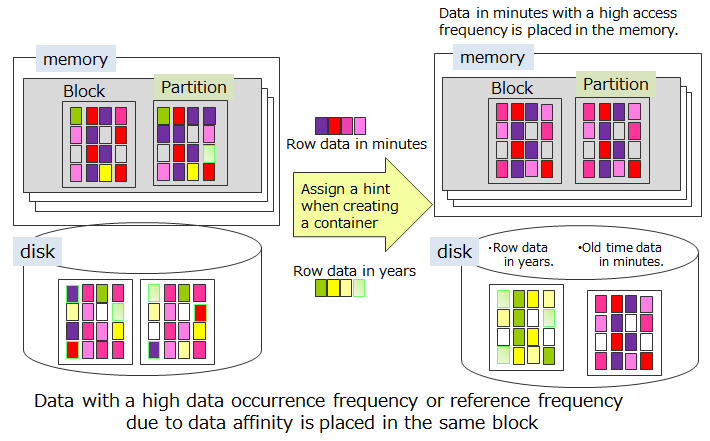
Data with the same hint information is placed in the same block as much as possible. Hint information is set depending on rate of data updates and data reference. For example, consider the data structure when system data is registered, referenced or updated by the following operating method in a system that samples and refers to the data on a daily, monthly or annual basis in a monitoring system.
- Data in minutes is sent from the monitoring device and saved in the container created on a monitoring device basis.
- Since data reports are created daily, one day's worth of data is aggregated from the data in minutes and saved in the daily container
- Since data reports are created monthly, daily container (table) data is aggregated and saved in the monthly container
- Since data reports are created annually, monthly container (table) data is aggregated and saved in the annual container
- The current space used (in minutes and days) is constantly updated and displayed in the display panel.
In GridDB, instead of occupying a block in a container unit, data close to the time is placed in the block. Therefore, refer to the daily container (table) in 2., perform monthly aggregation and use the aggregation time as a ROWKEY (PRIMARY KEY). The data in 3. and the data in minutes in 1. may be saved in the same block.
When performing yearly aggregation (No.4 above) of a large amount of data, the data which need constant monitoring (No.1) may be swapped out. This is caused by reading the data, which is stored in different blocks (No.4 above), into the memory that is not large enough for all the monitoring data.
In this case, hints are provided according to the access frequency of containers (tables), for example, per minute, per day, and per month, to separate infrequently accessed data and frequently accessed data from each other to place each in a separate block during data placement.
In this way, data can be placed to suit the usage scene of the application by the data affinity function.
[Note]
- Data affinity has no effect on containers (tables) placed in different partitions.
To place specific containers (tables) in the same partition, use the node affinity function.
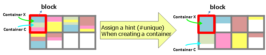
Placing each container (table) in a separate block
This is a function to occupy blocks on a per container (table) basis. Allocating a unique block to a container enables faster scanning and deletion on a per container basis.
As hint information, set a special string "#unique" to property information when creating a container. Data in a container with this property information is placed in a completely separate block from data in other containers.
[Note] There is a possibility that the memory hit rate when accessing multiple containers is reduced.
Node affinity
Node affinity refers to a function to place closely related containers or tables in the same node and thereby reduce the network load when accessing the data. In the GridDB SQL, a table JOIN operation can be described, such that while joining tables, it reduces the network load for accessing tables each placed in separate nodes of the cluster. While node affinity is not effective for reducing the turnaround time as concurrent processing using multiple nodes is no longer possible, it may improve throughput because of a reduction in the network load.
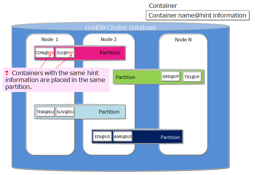
To use the node affinity function, hint information is given in the container (table) name when the container (table) is created. A container (table) with the same hint information is placed in the same partition. Specify the container name as shown below.
- Container (table) name@node affinity hint information
The naming rules for node affinity hint information are the same as the naming rules for the container (table) name.
[Note]
- This function cannot be used when table partitioning is in use.
Change the definition of a container (table)
You can change container definition including that of column addition after creating a container. Operations that can be changed and the interfaces to be used are given below.
| When the operating target is a single node | NoSQL API | SQL |
|---|---|---|
| Add column(tail) | ✓ | ✓ |
| Add column(except for tail) | ✓ (*1) | ✗ |
| Delete column | ✓ (*1) | ✗ |
| rename column | ✗ | ✓ |
- (*1) If you add columns except to the tail or delete columns, the container is recreated internally. Therefore, it takes a long time to operate the container whose data amount is large.
- Operations that are not listed above, such as changing the name of a container, cannot be performed.
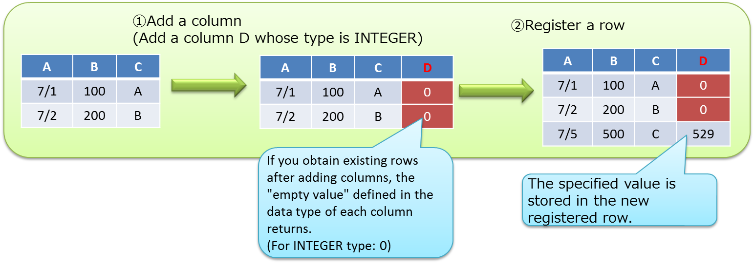
Add column
Add a new column to a container.
NoSQL API
Add a column with GridStore#putContainer.
[Example program]
java// Get container information ContainerInfo conInfo = store.getContainerInfo("table1"); List<ColumnInfo> newColumnList = new ArrayList<ColumnInfo>(); for ( int i = 0; i < conInfo.getColumnCount(); i++ ){ newColumnList.add(conInfo.getColumnInfo(i)); } // Set a new column to the tail newColumnList.add(new ColumnInfo("NewColumn", GSType.INTEGER)); conInfo.setColumnInfoList(newColumnList); // Add a column store.putCollection("table1", conInfo, true);
SQL
- Add a column using the ALTER TABLE syntax.
If you obtain existing rows after adding columns, the "empty value" defined in the data type of each column as a additional column value returns. See Container<K,R> of a "GridDB Java API Reference" for details about the empty value. (In V4.1, there is a limitation "Getting existing rows after addition of a column results in NULL return from columns without NOT NULL constraint.") See the limitations page of "GridDB Release Notes" for details.
Delete column
Delete a column. It is only operational with NoSQL APIs.
- NoSQL API
- Delete a column with GridStore#putContainer. Get container information "ContainerInfo" from an existing container at first. Then, execute putContainer after excluding column information of a deletion target. See "GridDB Java API Reference" for details.
Rename column
Rename a container column, which is only operational with SQL.
Database compression/release function
Block data compression
When GridDB writes in-memory data to the database file residing on the disk, a database with larger capacity independent to the memory size can be obtained. However, as the size increases, so does the cost of the storage. The block data compression function is a function to assist in reducing the storage cost that increases relative to the amount of data by compressing database files (data files). In this case, flash memory with a higher price per unit of capacity can be utilized much more efficiently than HDD.
Compression method
When the data on memory is exported to database files (data files), compression is performed for each block, which represents the write unit in GridDB. The vacant area of Linux's file space due to compression can be deallocated, thereby reducing disk usages.
Supported environment
Since block data compression uses the Linux function, it depends on the Linux kernel version and file system. Block data compression is supported in the following environment.
- OS: RHEL / CentOS 7.9 and later, Ubuntu Server 20.04
- File system: XFS
- File system block size: 4 KB
If block data compression is enabled in other environments, the GridDB node will fail to start.
Configuration method
The compression function needs to be configured in every nodes.
- Set the following string in the node definition file (gs_node.json) /dataStore/storeCompressionMode.
- To disable compression functionality: NO_COMPRESSION (default)
- To enable compression functionality: COMPRESSION
- The settings will be applied after GridDB node is restarted.
- By restarting GridDB node, enable/disable operation of the compression function can be changed.
[Note]
- Block data compression can only be applied to data files. Checkpoint log files, transaction log files, backup files, and the data on memory in GridDB are not subject to compression.
- Block data compression makes data files into sparse files.
- Even when the compression function is enabled, data that has already been written to data files cannot be compressed.
Deallocation of unused data blocks
The deallocation of unused data block space is the function to reduce the size of database files (actual disk space allocated) by deallocating the Linux file blocks in the unused block space in database files (data files).
Use this function in the following cases.
- A large amount of data has been deleted
- There is no plan to update data and it is necessary to keep the DB for a long term.
- The disk becomes full when updating data and reducing the DB size is needed temporarily.
The processing for the deallocation of unused blocks, the support environment and the execution method are explained below.
Processing for deallocation
During the startup of a GridDB node, unused space in database files (data files) is deallocated. Those remain deallocated until data is updated on them.
Supported environment
The support environment is the same as the block data compression.
Execution method
Specify the deallocation option, --releaseUnusedFileBlocks, of the gs_startnode command, in the time of starting GridDB nodes.
Check the size of unused space in database files (data files) and the size of allocated disk space using the following command.
- Items shown by the gs_stat command
storeTotalUse
The total data capacity that the node retains in data files (in bytes)
dataFileAllocateSize
The total size of blocks allocated to data files (in bytes)
It is desired to perform this function when the size of allocated and unused blocks is large (storeTotalUse << dataFileAllocateSize).
[Note]
- This function is available only for data files. Unused space in checkpoint log files, transaction log files and backup files is not deallocated.
- Deallocation of unused data blocks makes data files into sparse files.
- This function can reduce the disk usage in data files, but can be disadvantageous in terms of performance in that by making data files into sparse files, fragmentation is more likely to occur.
- The start-up of GridDB with this function may take more time than the normal start-up.